Python source code: plot_fft.py

import matplotlib.pyplot as plt
from scipy import fftpack
from scipy import signal

from dyna import forced_pendulum

omega = 2./3

dt = 2*np.pi / omega / 100

tf = 1000

acc_factors = [1, 1.07]


t, theta_0, theta_dot_0 = forced_pendulum(tf, dt, np.pi/3, 0,
                        q=0.5, acc=acc_factors[0], omega=omega)

t, theta_1, theta_dot_1 = forced_pendulum(tf, dt, np.pi/3, 0,
                        q=0.5, acc=acc_factors[1], omega=omega)

time_mask = t > 400

theta_0 = theta_0[time_mask]
theta_1 = theta_1[time_mask]

theta_0 -= theta_0.mean()
theta_1 -= theta_1.mean()

hann = signal.hanning(len(theta_0))
theta_0 *= hann
theta_1 *= hann

fft_theta_0 = fftpack.fft(theta_0)
freq = fftpack.fftfreq(len(theta_0), dt)

fft_theta_1 = fftpack.fft(theta_1)

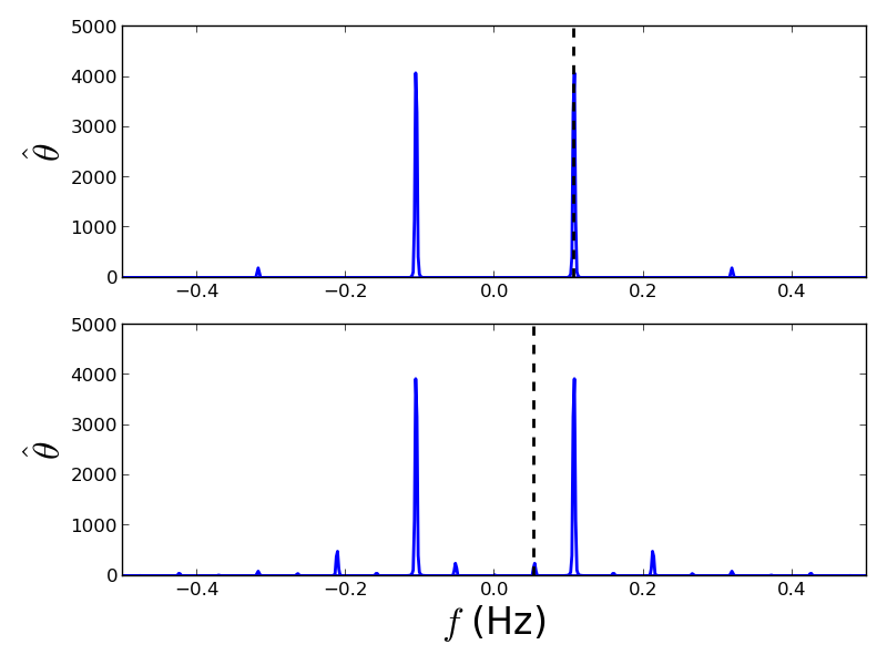
f_driving = 2./ 3 * 1./ (2 * np.pi)

plt.figure()
plt.subplot(211)
plt.plot(freq, np.abs(fft_theta_0), lw=2)
plt.axvline(f_driving, ls='--', color='k', lw=2)
plt.xlim(-0.5, 0.5)
plt.ylim(0, 5000)
plt.ylabel(u'$\hat{\\theta}$', fontsize=24)
plt.subplot(212)
plt.plot(freq, np.abs(fft_theta_1), lw=2)
plt.axvline(f_driving / 2, ls='--', color='k', lw=2)
plt.xlim(-0.5, 0.5)
plt.ylim(0, 5000)
plt.xlabel(u'$f$ (Hz)', fontsize=24)
plt.ylabel(u'$\hat{\\theta}$', fontsize=24)

plt.tight_layout()

plt.show()

Total running time of the example: 0.00 seconds